Quality Control of surface defects and inclusions using Deep Learning Image Segmentation
Abstract
Automatic detection of abnormalities by machine learning has become an interesting and promising research field that has a very high and direct impact on the field of visual inspection. Deep learning techniques have emerged as the best approach to this task. Deep learning techniques can deliver a model that can detect surface anomalies simply by training them on a dataset of images.
Introduction
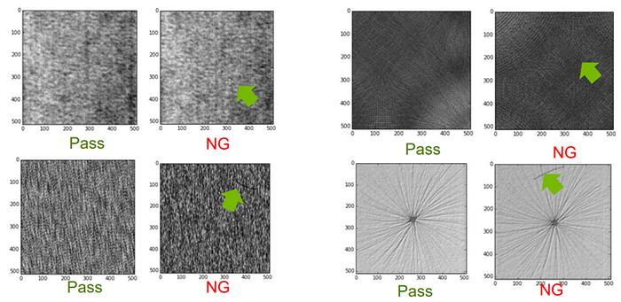
In several industries, an inspection of the surface of a finished product or inspection of impurities in materials via SEM/EDX is one of the steps for quality control. Often, this inspection process involves quality personnel inspecting the surfaces manually.
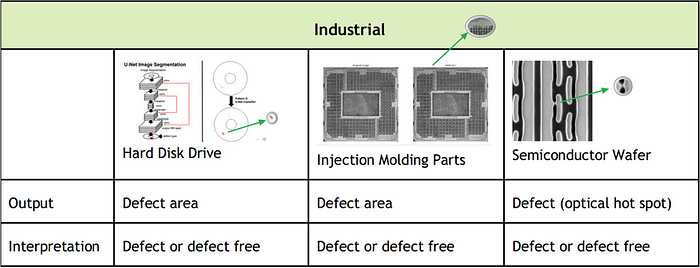
This requires training a QC inspector to identify a whole range of complex defects. This is time-consuming, inefficient, and can contribute to production wait times and even occasional misclassification of a defect that can lead to customer complaints or field failures leading to product recalls. In the past, traditional image processing methods were sufficient to solve these problems (Paniagua et al., 2010; Bulnes et al., 2016). However, the Industry 4.0 paradigm tends toward generalizing production lines that require rapid adaptation to new products (Oztemel and Gursev2018). In this article, I have explored 2D Convolution Neural Network-based U-Net Architecture to detect defects.
U-Net
The UNET was developed by Olaf Ronneberger et al. for BioMedical Image Segmentation. The architecture contains two paths. The first path is the contraction path (also called the encoder) which is used to capture the context of the image. The encoder is just a traditional stack of convolutional and max-pooling layers. The second path is the symmetric expanding path (also called the decoder) which is used to enable precise localization using transposed convolutions. Thus it is an end-to-end, fully convolutional network (FCN), i.e., it only contains Convolutional layers and does not contain any Dense layer because of which it can accept images of any size.
In the original paper, the UNET is described as follows:

Here’s a good article on U-Net implementation:
https://towardsdatascience.com/understanding-semantic-segmentation-with-unet-6be4f42d4b47
Dataset
This dataset is artificially generated but similar to real-world problems. It consists of multiple data sets, each consisting of 1000 images showing the background texture without defects and 150 images with one labeled defect each on the background texture. The images in a single data set are very similar, but each data set is generated by a different texture model and defect model.
Not all deviations from the texture are necessarily defects. The algorithm will need to use the weak labels provided during the training phase to learn the properties that characterize a defect.
Python Libraries:
matplotlibxmltodictsklearntensorflowscipy
Cloning the Repository
Clone the repository to a local folder:
git clone https://github.com/AdarshGouda/Surface-Defect-Detection.gitcd Surface-Defect-Detection
The helper functions will aid in locating the defect and masking it with an eclipse located in the ./utils folder. This folder and its contents will be imported as needed in the code below.
Download the dataset and unzip it:
wget https://resources.mpi-inf.mpg.de/conference/dagm/2007/Class1_def.zipThe dataset takes up to a few minutes to download, depending on your network connectivity.
unzip -q Class1_def.zip -d .Let's take a look at the images in the ./Class1_def folder.

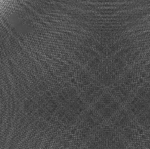
Notice the defect in the top left corner in image 1.png. The helper function in the ./utils folder will help in locating these defects in an image and create a corresponding mask as a label.
The following code block in Surface-Defect-Detection.ipynb file will plot the segmentation label to any image you might want to test out. Here, I’ve tested the first image 1.png
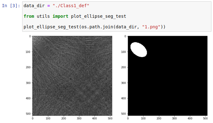
The load_images_masks() function in the DataIO.py script takes in the raw image file from the Class1_def folder and returns both the image and its segmented label.

As seen in the above output, there are 150 total images of size 512 x 512 and 1 channel (grayscale images and not RGB)
Next, let's take a look at the first X and y data points.

As seen above, the segmented label is correctly identifying the location of the defect in the original image.
Train-Test Split

Define a distilled version of U-net to make computation and training simpler.


Loss Function and the Smooth Dice Coefficient:
A popular loss function for image segmentation tasks is based on the Dice coefficient, which is essentially a measure of overlap between two samples. This measure ranges from 0 to 1, where a Dice coefficient of 1 denotes perfect and complete overlap. The Dice coefficient was originally developed for binary data and can be calculated as:

where |A∩B| represents the common elements between sets A and B, and |A||A| represents the number of elements in set A (and likewise for set B).
For the case of evaluating a Dice coefficient on predicted segmentation masks, we can approximate |A∩B||A∩B| as the element-wise multiplication between the prediction and target mask and then sum the resulting matrix.

Because our target mask is binary, we effectively zero out any pixels from our prediction which are not “activated” in the target mask. For the remaining pixels, we are essentially penalizing low-confidence predictions; a higher value for this expression, which is in the numerator, leads to a better Dice coefficient.
In order to quantify |A| and |B|, some researchers use the simple sum, whereas other researchers prefer to use the squared sum for this calculation. I don’t have the practical experience to know which performs better empirically over a wide range of tasks, so I’ll leave you to try them both and see which works better.

In case you were wondering, there’s a 2 in the numerator in calculating the Dice coefficient because of our denominator “double counts” the common elements between the two sets. To formulate a loss function that can be minimized, we’ll simply use 1−Dice1−Dice. This loss function is known as the soft Dice loss because we directly use the predicted probabilities instead of thresholding and converting them into a binary mask.
With respect to the neural network output, the numerator is concerned with the common activations between our prediction and target mask, whereas the denominator is concerned with the number of activations in each mask separately. This has the effect of normalizing our loss according to the size of the target mask such that the soft Dice loss does not struggle learning from classes with lesser spatial representation in an image.
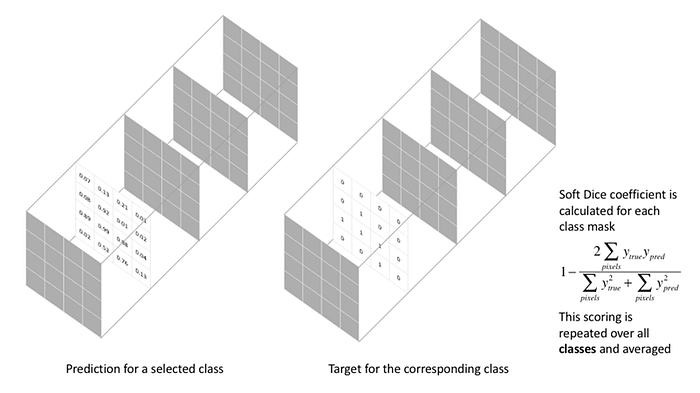
Let's define the smooth_dice_coeff() function to calculate losses and compile the model:

Train
I have chosen a batch size of 10 with 60 epochs. The batch size of 10 helped me run the training on RTX3070 (laptop).


Learning Curves
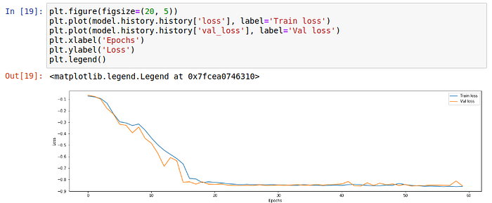
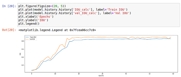
The learning curves aren't too bad. There are no signs of underfitting or overfitting — which is a good sign.
Testing (Prediction)

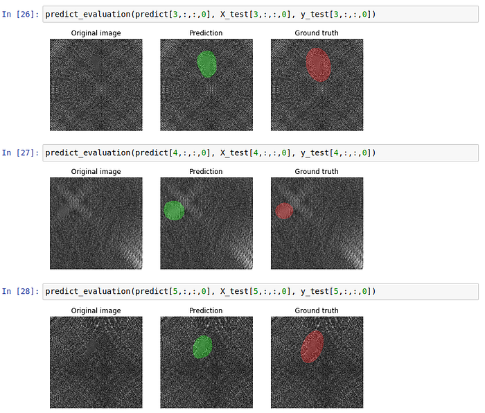
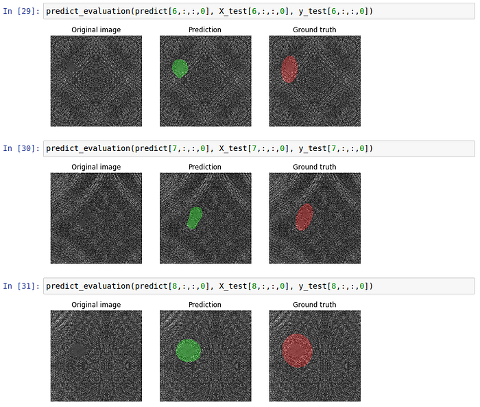
We will use the function predict_evaulation() to check our results on the few images in the Test set.

Conclusion
This exercise was more of a proof of concept. The training images were artificially generated. In the real world, it is possible that the images received from cameras or digital microscopes may not have similar contrast or brightness values which may make it difficult to detect defects. Using data augmentation techniques during training might help in preparing a trained model for real industrial applications. For the purposes of this article, the results were better than what I thought they would be.
References:
1. U-Net: Convolutional Networks for Biomedical Image Segmentation https://arxiv.org/abs/1505.04597
2. Tabernik, D., Šela, S., Skvarč, J. et al. Segmentation-based deep-learning approach for surface-defect detection. J Intell Manuf 31, 759–776 (2020). https://doi.org/10.1007/s10845-019-01476-x
3. NVIDIA End-to-End Deep Learning Platform
4. The One Hundred Layers Tiramisu: Fully Convolutional DenseNets for Semantic Segmentation https://arxiv.org/abs/1611.09326
5. Edge AI in Smart Manufacturing: Defect Detection and Beyond
Appendix: Code for Complete U-net
<Attach>

