Exploring Deep Neural Networks for Design Optimization of Engineering Problems
Abstract
Modeling & Simulation has played a significant role in improving design cycle time with extensive use of FEA and CFD solvers that implement various methods for solving differential equations. However, as the problem domain becomes larger with increasing degrees of freedom and complex boundary conditions, the computational time needed to solve the system of equations may range from several hours to days and even weeks. With such cycle times between simulations, optimizing the model even slightly will need the simulation to be run from the start.
In recent times, machine learning algorithms are becoming increasingly popular in several fields. It has been successfully demonstrated over the decade that if ML models are properly chosen and trained, the models perform exceptionally well from conventional techniques.
This article provides a basic understanding of how Neural Networks can be used to significantly reduce the overall computation time and complement modeling and simulation techniques. An example of a cantilever beam in harmonic oscillation is presented using Python and TensorFlow.
1. INTRODUCTION
Artificial Neural Networks are being used to solve different types of large data-related problems in many fields. The reason for its popularity is that ANN provides an alternative to conventional mathematics, algorithms, and methodologies where the inherent limitations lead to unsatisfactory solutions. Such problems are usually complex and perhaps the relationships between various parameters and features involved in such problems are not adequately defined or fully understood.
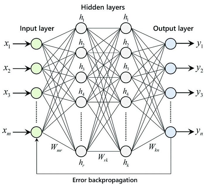
ANNs are built like the human brain, with neurons or nodes interconnected like a web. Figure 1 shows a basic structure of a Fully-Connected Neural Network. Here it can be seen that the set of input features (X) is passed through different neurons, whose output is a non-linear function of the contents of the previous layer, Figure 2. The process is repeated until a set of output units 𝐘 is obtained.


The most common types of activation functions employed in Machine Learning can be found in Figure 3. An important property of the neurons presented in Figure 2 is that they have proven to fulfill the Universal Approximation Theorem. This theorem states that, if there exists a function 𝐘 = 𝑓(𝐗), then a sufficiently large neural network can approximate any such function.

Each of these activation functions has its own advantages and disadvantages. Hence, an activation function is deployed based on several factors such as the nature of the problem (classification or regression), the quality of data available for training, and the choice of a loss function.
2. Dataset for Training the ANNs

The dataset available will be split into a Train Set and a Test Set, typically in an 80:20 ratio. A model based on ANN will be only as good as the Train Set it is fed with. Hence, it is important that the data available is clean and treated in a way that only enhances the model performance on the Test set and does not underperform by overfitting the Train set. Each set will have features (Xs) and then the target variable (Y) which is predicted for Test Set.
A typical Machine Learning workflow involving the train and test dataset is shown in Figure 4.
In this paper, we will first generate data from a theoretical equation and also, we will use results for FEA simulations.
3. HARMONIC OSCILLATOR
Let’s take a look at one of the most fundamental systems — a one-dimensional harmonic oscillator. When the system is displaced from its equilibrium, it experiences a reaction force that is proportional to the displacement.
Let’s dive into generating a harmonic spectrum using the analytical equation. Then we will split the data into Train and Test Set. We will then train the ANN on the Train Set and then predict the amplitude on the Test Set.
We will be using TensorFlow to create ANN model, Matplotlib to plot the graphs, Numpy to handle arrays, and Pandas to handle the dataset from the CSV file.
[1] Importing essential python libraries

[2] Enabling GPU memory growth. (I am running this ML on an RTX 3070 with CUDA support.)

[3] Defining a function to generate amplitude data for a given range of frequency and intervals.

[4] Assigning parameters

[5] Generating amplitudes

[6] Plotting Amplitude vs Frequency


The amplitude is plotted on a log scale, hence the use of plt.semilogy()
The amplitude is now stored in an array “a” and the corresponding frequency is stored in array “f”
[7] Splitting Train and Test Data using sklearn. 20% Test Set

Clearly, our input is the frequency and we will be predicting corresponding amplitude.
[8] Creating a Sequential ANN Model

Let me explain the above code in some detail. We are using the Sequential model from Keras which now is embedded into TensorFlow 2.0 onwards.
The first line in the code is to declare a variable name for our model.
The second line is adding an Input Layer to our model. Refer to Figure 1, this is the first layer in our neural network. The shape of our input is 1 since we just have a one-dimensional array “f” as our input.
The 3rd, 4th, and 5th lines in the code are adding 3 hidden layers with 30 neurons each with tanh activation function. Refer to Figure 2 to understand this better.
The 6th line is adding the output layer. Since we are interested in only one output, i.e., amplitude, we just need one node in our input layer. The activation function is “linear” since our output is a raw number ranging from -inf to +inf.
Now, I had to perform hyperparameter tuning to get the best setup of this model. We can use wrappers available in Keras to use GridSearch or RandomSearch from sklearn with Cross-fold validation to get the best hyperparameters for our model.
The 7th line in the code is creating an instance Stochastic Gradient Descent (SGD) optimizer to find the global minima of our cost-function. The learning rate is set at 0.01 and Nesterov’s accelerated gradient descent is enabled with momentum set at 0.9. Again, these are hyper-paraments the need to be iteratively tuned to get the best out of your model.
The last line is basically compiling the model with the hyperparameters and the layers. This also where we declare our cost function and the optimizer. “mse” stands for Mean Squared Error which my choice of cost-function for this problem.
[9] We now train our model on the Train Set

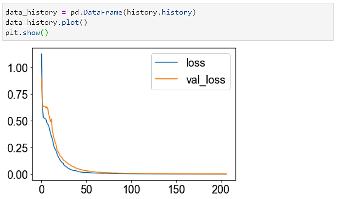
The epochs are basically a number of times the model will iterate to minimize the error and find a global minimum for our cost function which is mean squared error in our case. The validation split is to enable 10% of the Train Set data to use for validating the performance. The callback then uses the performance of the model on validation to stop the epochs are a point where there is no further improvement in the performance for 10 subsequent iterations. Assigning the history of the epochs to a variable called “history” to later analyze the performance of the training.
[10] Evaluating the losses on the Test Set

The losses are very low. This is good!
[11] Plotting the history of the epochs

As you can see, although we declared 1000 epochs, the training stopped at a little over 200 epochs given that the losses on the validation set were not improving for the last 10 epochs.
[12] Let's use the model to predict the amplitude on our Test Set that we set aside for our data.

[13] Let's find the R2-Score for our model.

That’s an amazing R2 value! Closer to 1 is the best!
[14] Let's plot the log of predicted amplitude vs the ground truth


Superb results! The predictions from our model perfectly fit the analytical results we had generated in step [6]. There is some deviation in the far right. Perhaps we can increase the number of neurons in each hidden layer to allow the model to learn better.
Let’s take this up a notch and develop an ANN model for a 3D problem — harmonic response of a Cantilever Beam.
4. Cantilever Beam Harmonic Response
Let’s consider a steel cantilever beam of square cross-section, reduced-damping, and calculate its response for a harmonically varying external load. The beam geometry described below.


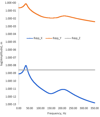
The harmonic response is run for 0–350Hz frequency range with 10000 intervals and simulation is run with Ansys Workbench solver. The load 1000N is applied in the negative Y direction. As seen in Figure 6, the Z response is pretty much zero.

The results — response X, Y, and Z amplitudes of the beam at each frequency is exported into a CSV file. This data is then imported into Python and will be our entire dataset to train and test our neural network model.
Let’s work on our ANN model now.
[15] Import the CSV file into python.

The “Frequency” is our Input (X) and the 3 amplitude values are Targets (Y)
[16] Prepare the Train & Test Set

[17] Build the model. Notice that this time we have used Adam optimizer which is another popular optimizer for ANNs.

[18] Train the model

[19] Evaluate the model

Notice that the loss is super low. This is good!
[20] Plot the epoch history

[21] Predict the amplitude values on Test Set

[22] Plot the predicted results and results from Ansys


There it is! The model beautifully predicts amplitudes in all the directions at one intense for any given frequency.
5. CONCLUSION
The real applications will be much more complex than the example presented here, of course. Given the versatility of Artificial Neural Networks and Deep Learning methodologies, the approach discussed here can then be advanced to solve more realistic problems. By training neural networks, there are tremendous possibilities to reduce the design optimization time by running few cases using FEA or CFD and then training a neural network to predict other possible cases to get the best of both worlds. Yet another area of interest, especially for CFD, is the Convolution Neural Networks that can detect patterns in the flow field.
