Predicting Oil Production Trends using Deep Learning to Appraise Oil Wells

10 min readAug 8, 2022

1. Introduction

The production profiles of oil wells can be complicated, driven by reservoir physics, defined by a variety of operational events, and obscured by data noise. This makes it difficult to value an oil company accurately. Most of the time, petroleum engineers can interpret oil wells' production profiles, comprehend their underlying behavior, predict their production, and spot areas for performance enhancement. However, this analytical process consumes time. This creates an opportunity to assess a broad array of previously unknown options to enhance the analytical procedure of predicting production trends. In this study, an investigation is carried out to assess if oil well activity can be understood and predicted using deep learning methods, which are well-known to be efficient in pattern recognition and object categorization.

2. Dataset

The original data is stored in a spreadsheet containing information on seven drilling sites with the date of the measurement taken, the field name, formation type, well name, oil production, water production, and gas production[3]. Each of the seven sites contains several Wells, and each Well is identified by its Well name. The Well name is generated using the first two letters of the field name, the first two letters of the formation type, and an index. Every Well contains data for oil, water, and gas production for every month it has been drilled, as indicated by the date. Only the oil production data is considered in this analysis. However, the given Dataset has a few inherent problems: each site varies in the number of Wells, each Well varies in the amount of data associated with it, and data points were often zeroed out (i.e., missing) or very large, probably incorrectly recorded.

3. Preprocessing

Let's take a look at the files in the ./data directory.

There are 7 CSV files from 7 different drilling sites. Let's import them into a Pandas DataFrame.

The above line of code concatenates the data from all 7 CSV files into one DataFrame. Let's take a look at the contents of the Dataset.

The Dataset includes information on seven drilling locations, including the date the measurement was made, the field name, formation type, well name, and the amount of oil, water, and gas produced. There are multiple wells at each of the seven locations; each Well is identifiable by its unique Well name. The first two letters of the field name, the first two letters of the formation type, and an index are used to create the Well name. Every Well provides information on each month's gas, water, and oil production since it was drilled, as indicated by the date.

Only the oil production data is considered for this study [3] by extracting the Well_Name and Oil columns from the Dataset.

There are a total of 114529 entries (or rows) in the Dataset. Let's check if there are any NaN entries.

Fortunately, there are no null entries.

Let's count the number of unique Wells in the Dataset.

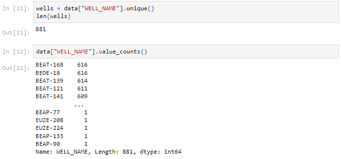
There are 881 unique Wells in the Dataset. The number of Wells at each location clearly varies, as does the quantity of data that is available for each Well.

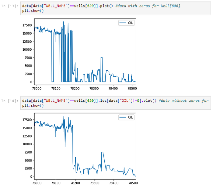
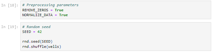
Many data points are zeroed out (i.e., missing) or extremely big, suggesting that they were probably recorded improperly. This issue was rectified by excluding the blanked-out or missing data points. These data points showed periods when the Well was shut off or when data wasn't collected; they reflect inaccurate oil production statistics for the time series and point to periods when the Wells' condition was probably not going to change over time. These missing or zeroed points cease to be useful for training and prediction for the time series of oil wells. The remaining non-zero points are combined to produce a time series free of erroneous zeros that could impede training.

Below a dictionary is created with each Well as a unique Key, and the non-zero Oil production float value is appended as an array to a given Well (Key).

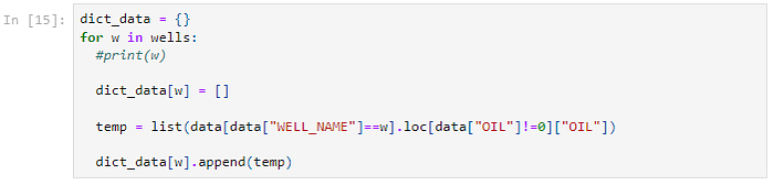
Let's take a peek at the dictionary dict_data.

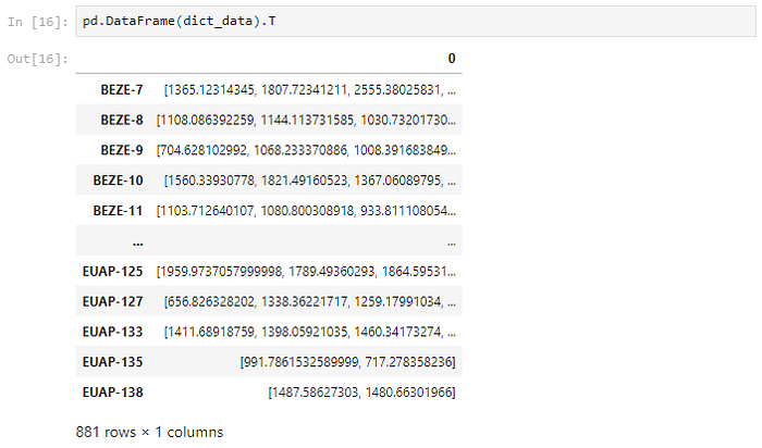
Now, we have a dictionary of all wells and the corresponding oil production numbers over a period of time. But, the amount of data available for each Well varies. This creates a problem for a neural network that typically takes a fixed input size.

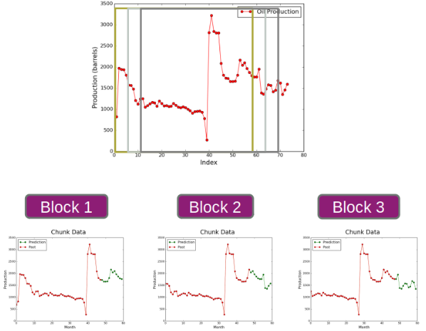
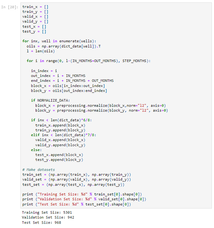
This is why data blocks of equi-sized data points are created by sliding a window of 60 data points with a step size of 6. The 60 data points are further distributed as the first 48 months of data for training and the immediately following 12 data points as test points [3].

The oil production numbers significantly vary from pocket to pocket. Each data block needs to be normalized to maintain a sensible scale which will help in effective training.

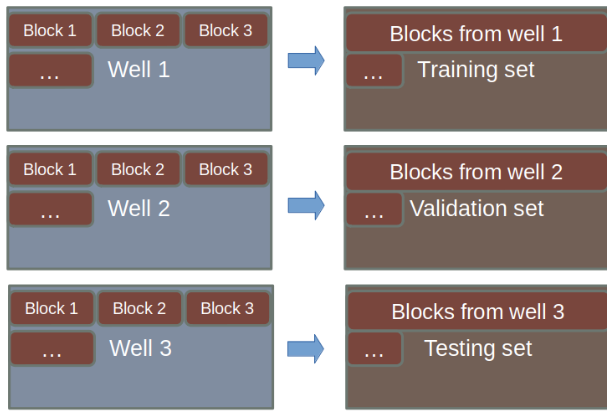
Next, the data is split into a train, test, and validation set.

4. Experiments

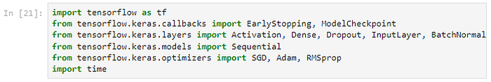
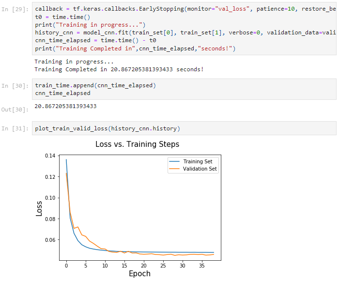
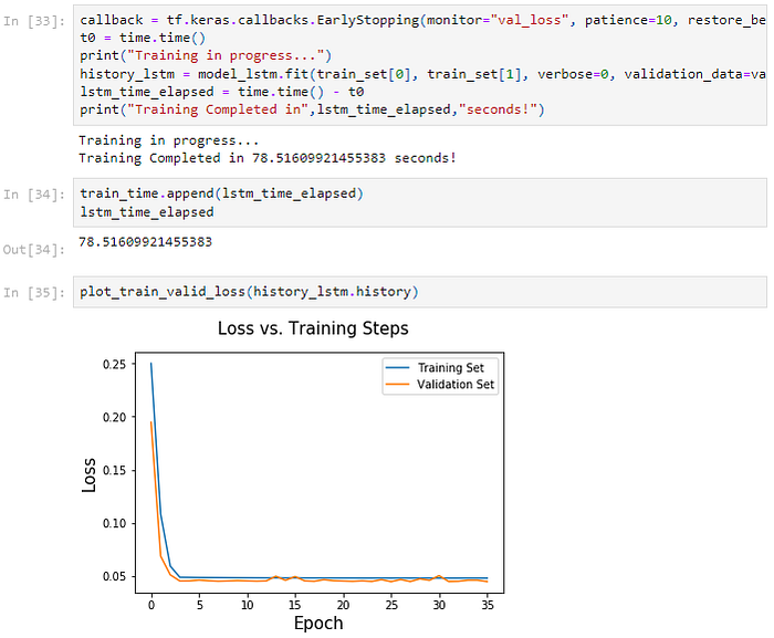
To run experiments, Multilayer Perceptron, 1D Convolution Neural Network, and LSTMs are considered. SGD, ADAM, and RMSprop optimizers were tried and it was found that RMSprop performs better with smaller batch sizes. MAE and MSE loss functions were considered for the analysis. Both the loss functions perform reasonably well. I used MSE in my experiments because they seem to converge faster. I also found that a learning rate of 0.0001 is apt for the Dataset. I also used EarlyStopping to stop the model from overfitting with a patience value of 10 while monitoring validation losses.

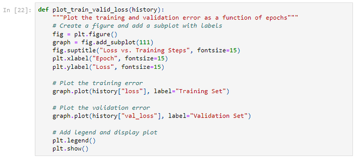
Below is a helper function to plot the loss history from training.

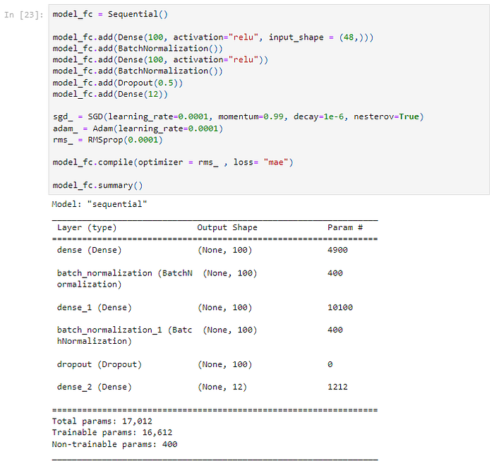
4.1 Multilayer Perceptron

The multilayer perceptron (MLP) is the simplest form of a deep, fully connected network. This feedforward model means that information flow is always directed towards the output layer. MLPs operate by mapping sets of input data onto sets of output data. It has been shown that they can serve as universal function approximators. MLPs have an input layer whose values are determined by the input samples, at least one hidden layer derived from previous layers, and an output layer derived from the last hidden layer. Each neuron in the input and hidden layers has a forward-directed connection to each neuron in the next layer. A non-linear activation function at each neuron introduces non-linearity to the neural network.

MLPs attempt to model the human brain in a very simple fashion. Each neuron in the network receives data from every neuron in the previous layer, and each of these inputs is multiplied by an independent weight. The weighted inputs are summed and are then sent through an activation function which is usually designed to scale the output to a fixed range of values. The outputs from each neuron can then be fed into the next neural network layer in the same fashion.

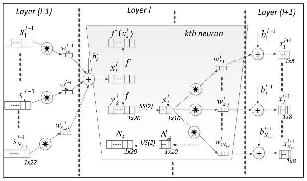
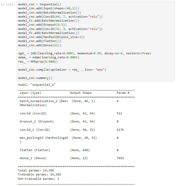
4.2 1D Convolution Net

As in the conventional 2D CNNs, the input layer is a passive layer that receives the raw 1D signal, and the output layer is an MLP layer with the number of neurons equal to the number of classes. Three consecutive CNN layers of a 1D CNN are presented in the Figure below. As shown in this Figure, the 1D filter kernels have a size of 3, and the sub-sampling factor is 2, where the kth neuron in the hidden CNN layer, l, first performs a sequence of convolutions, the sum of which is passed through the activation function, followed by the sub-sampling operation. This is the main difference between 1D and 2D CNNs, where 1D arrays replace 2D matrices for both kernels and feature maps. As a next step, the CNN layers process the raw 1D data and "learn to extract" such features which are used in the classification task performed by the MLP layers. As a consequence, both feature extraction and classification operations are fused into one process that can be optimized to maximize classification performance. This is the major advantage of 1D CNNs, which can also result in a low computational complexity since the only operation with a significant cost is a sequence of 1D convolutions, which are simply linear weighted sums of two 1D arrays. Such a linear operation during the Forward and Back-Propagation operations can effectively be executed in parallel.

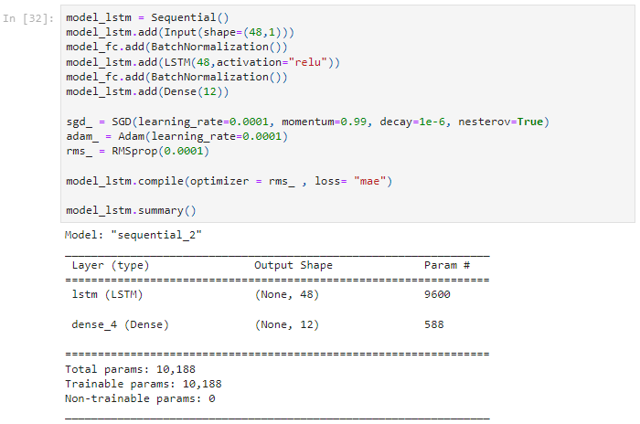
4.3 LSTM Recurrent Neural Network

LSTM is a modified RNN architecture developed by Hochreiter and Schmidhuber in 1997. LSTM addressed the vanishing gradient problem and allows the storage of information for an extended time period.

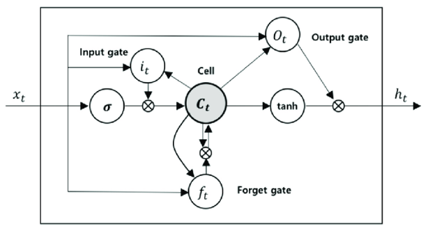
LSTM consists of a standard RNN, additional self-connected memory cells, and three multiplicative units — the input, output, and forget gates — that equivalently write, read, and reset information within the model's cells. In an LSTM network, memory cells displayed in the Figure below replace summation units in the hidden layer. These memory cells contain the three multiplicative gates, enabling the LSTM memory cells to store and access information over long periods. The gates control the amount of information fed into the memory cell at a given time step.

By refraining from traditional RNN methods of overwriting new content at each timestep, the LSTM can effectively decipher important features and carry that information over a long distance.

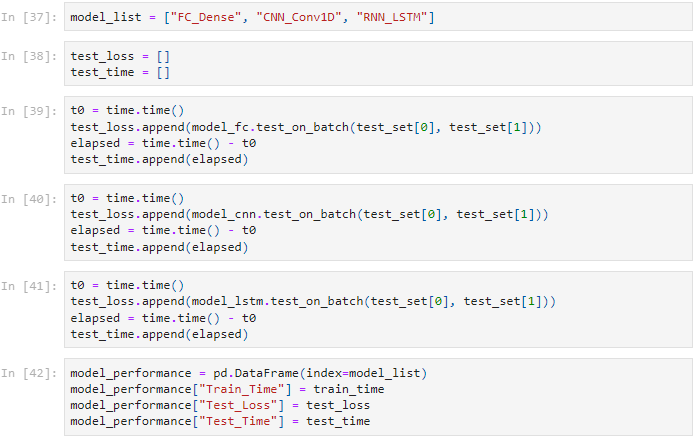
5. Performance and Prediction

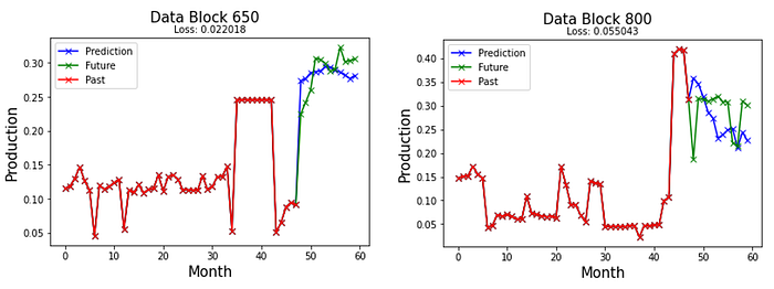
5.1 MLP Model prediction on Test Block Data 650 & 800

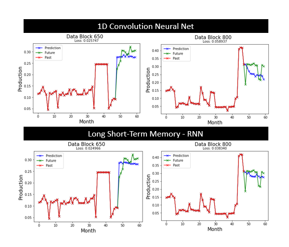
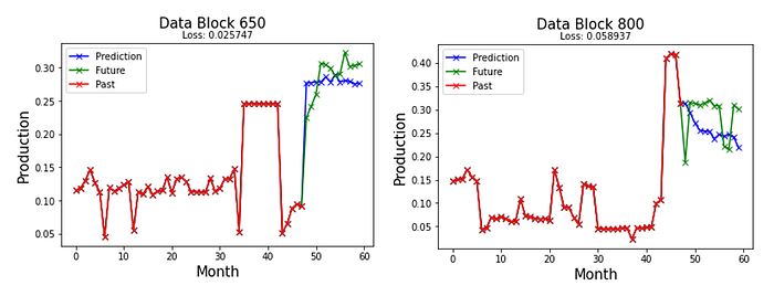
5.2 Conv1D Model prediction on Test Block Data 650 & 800

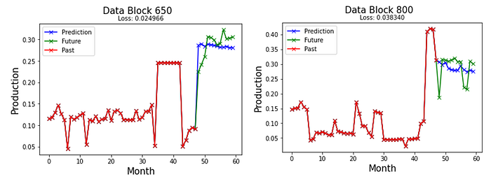
5.3 LSTM Model prediction on Test Block Data 650 & 800

6. Results & Discussions

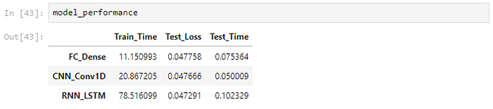
The LSTM model performs well on the test set. However, the MLP model is the fastest to Train on, with losses very close to that of the Conv1D and LSTM models.

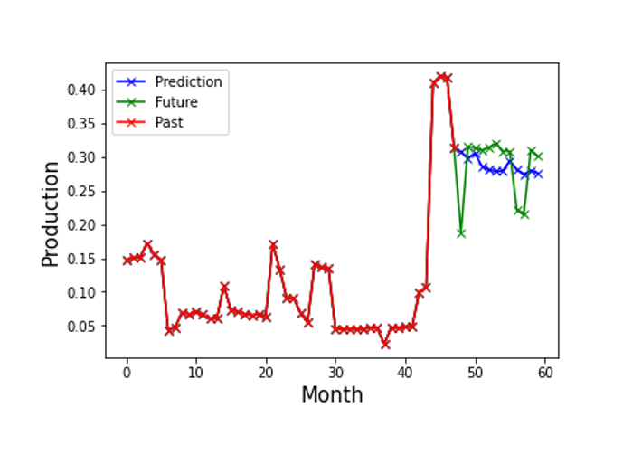
The models tend to predict downward trends better than upward trends. Also, all the models fail to capture sudden spikes. However, they provide a reasonable prediction in most cases.

The deep neural network models could reasonably predict the data for twelve months of future oil production. Overall, despite being difficult to train, with many hyper-parameters to tune, deep learning is promising for many applications in the petroleum industry. The simplest of models is sufficient to set up a prediction model. These models' robust nature and ability to learn patterns in unlabeled data will make them a useful tool in the Oil sector.

References:

[1] Prasad, Sharat C., and Piyush Prasad." Deep Recurrent Neural Networks for Time Series Prediction." arXiv preprint arXiv:1407.5949 (2014).

[2] J. W. Taylor." Short-term electricity demand forecasting using double seasonal exponential smoothing." Journal of the Operational Research Society 54, no. 8 (2003): 799–805.

[3] Garcia, Janette & Tung, Albert & Yang, Michelle & Levy, Akash. (2015). Applying Deep Learning to Petroleum Well Data.

[4] Graves, Alex. Supervised sequence labeling with recurrent neural networks. Vol. 385. Heidelberg: Springer, 2012.

[5] Sutskever, Ilya, James Martens, George Dahl, and Geoffrey Hinton. " On the importance of initialization and momentum in deep learning." In Proceedings of the 30th international conference on machine learning (ICML-13), pp. 1139–1147. 2013.