Gesture Recognition From Video Sequences using Time Distributed 2DCNN-LSTM Architecture
GitHub Repository: https://github.com/AdarshGouda/2DCNN-LSTM
ABSTRACT
A ML method is explored that recognizes sign language from short video recordings and translates them into a natural language. These video sequences contain spatial and temporal features requiring a Convolution Neural Network (CNN) and a Recurrent Neural Network (RNN) in tandem. ImageNet trained VGG19 model is used as the CNN architecture to apply transfer learning to our dataset, and LSM is used to extract temporal information from the video sequences. The dataset chosen for this work contains gestures from the Argentinian Sign Language, of which 10 categories were chosen in the interest of computational time and memory constraints. The developed model achieved an accuracy of 96% over the set of video sequences.
BACKGROUND
The world has become more interconnected than ever before. People from different backgrounds and languages can communicate with each other instantaneously thanks to the development of real-time translation algorithms that have eroded longstanding language barriers. However, it has taken longer for this freedom of communication to reach the hearing impaired. The hearing-impaired use sign language as a system of communication using visual gestures and signs. The lag in developing sign language detection techniques is primarily due to the complexity of translating physical movements into verbal, or written, words.
Currently, the methods for recognizing hand signals are largely classified as sensor-based and vision-based. Sensor-based methods rely on sophisticated gloves worn by the person performing the hand gestures. Sensors in the gloves translate the movements into signals interpreted by computer applications into a form the general public can understand. The main disadvantage of sensor-based methods is that they depend on external hardware. On the other hand, vision-based methods depend solely on the interaction between humans and computers. The challenge is that sign language translation requires real-time hand gestures and body movement recognition. This means that applications need to perform classification through a high-volume video feed as input, making the task computationally heavy. Such challenges have impeded progress in sign language detection.
Unlike static images, videos contain both spatial and temporal information. This means that two types of networks are needed for this task. A CNN network was used to extract the spatial information, and an RNN network was used to recognize the information contained in the sequence. We utilized a TensorFlow package called Time Distributed CNN, which is a wrapper that is applied to each slice of an input. The video clips in the dataset were sorted into separate folders, one folder for each class. Each video contained a series of frames; however, the number of frames in each video varied. The exact number of frames was extracted from each video to maintain consistency. The frames were resized to constant size and then masked to extract only the hand gestures. The people performing the hand gestures wore red or green gloves to facilitate the masking process. A pretrained VGG19 was used for the CNN architecture to apply transfer learning to the task. This CNN model was used mainly as a feature extractor for each frame in a sequence. The extracted features were then put through the LSTM network and trained to recognize the various gestures.
This work aims to develop a lightweight model that would be easy to plug and play into various networking applications. By lightweight, we mean less demand for computing power and memory. This would minimize the impact on call quality and enable seamless real-time hand gesture translation. Such a model can be a plug-in to any video conferencing application for PC or mobile devices without requiring “heavy-duty” hardware.
The dataset consists of Argentinian Sign Language (LSA) gestures. This dataset was used because of the large number of samples available and the diverse set of classes. Furthermore, to simplify the problem of hand segmentation in the videos, the subjects wore fluorescent-colored gloves. This eliminated background effects, such as clothing and skin color, and allowed the model to focus on the shape of the hands. The diversity of the dataset was also a benefit in that all subjects were non-signers and right-handed and were taught how to perform the signs during the session recordings.
The Argentinian Sign Language database was created to have a dictionary to train and automatically detect the said sign language.
The dataset was created by Facundo Quiroga, a professor of Computer Science at the Instituto de Investigacion en Informatica — LIDI, in Argentina.
This database contains 3200 video samples of human sign language gestures from 64 different categories.
Each data instance is a visual recording of a person performing a hand gesture that indicates a sign (i.e., signing with their hands).
APPROACH
The dataset, when downloaded, contains 3,200 video files belonging to 64 classes. We have considered only the first 10 classes for all purposes in this project. These video files come in variable frame counts ranging from 60 to 240 frames. A fixed number of sequential frames (80 frames) are generated from these videos. The frames are passed into a pre-trained Convolution Neural Network to extract key features from each frame. The key features are then passed into an LSTM unit. The output from LSTM is passed to a softmax classifier to predict the class. Figure 1 illustrates an overview of the approach followed in this project.

SORTING THE DATASET
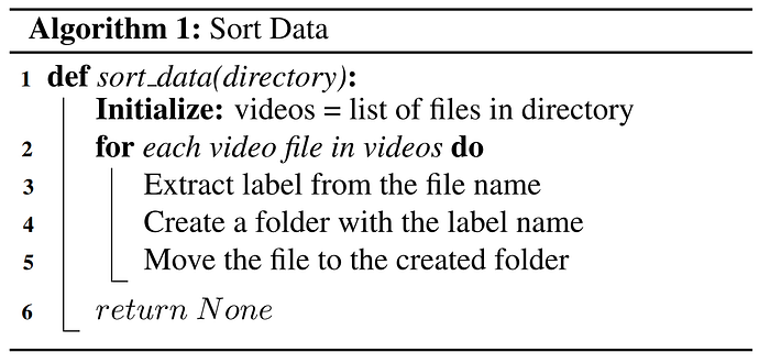
When downloaded from the site, the video dataset is not sorted according to the class labels. However, file names provide enough information to identify the class label of a given video file. Although it was possible to use the individual file as-is and load it into memory, the challenge was to be able to do this with limited RAM and GPU memory during training. For convenience and effectiveness in execution during training, it becomes imperative that the data be arranged systematically to choose the files belonging to the first 10 classes. The Python script sort_data.py creates folders for each class and moves the corresponding files into these. Algorithm 1 illustrates the implementation of this code. The python script is to be executed in the terminal.
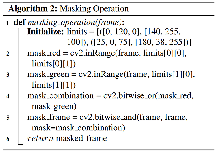
As briefly mentioned earlier, in this dataset, the subjects wore red gloves on their right hand and green on their left. This is very helpful in eliminating all the noises in the frames except for the hands, which are the most crucial aspect of signing. Each frame in the video was extracted, and then a color masking operation was applied to each frame using OpenCV that will convert the RGB frame into a grayscale image after performing inRange, bitwise_or, and bitwise_and operations. The python script to implement this masking operation can be found in mask.py. Algorithm 2 illustrates the masking operation. This StackOverflow Answer helped significantly in developing this masking operation. The challenge here was to find the exact values for the red and green masks, which took quite some time to figure out and implement using cv2.inRange.
FRAME EXTRACTION & PREPROCESSING
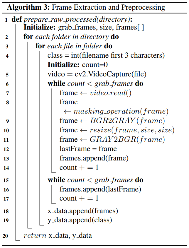
The videos in the dataset have varying duration. The frames of the video were extracted using Python’s OpenCV library. A fixed number of frames were extracted from the video files for consistent input dimensions to the CNN. The grab_frames variable in the config_default.yalm file could be set to desired frame counts during training. In this project, the frame count was set to 80 frames. If a video file had less than 80 frames, the last frame was repeatedly appended until 80 counts. The frame extraction code is part of the process_raw_data.py Python script illustrated in Algorithm 3. There are several ways to grab the frames. One explored implementation was to detect a change in pixel intensity by subtracting successive frames, and if the pixel intensity crosses a predetermined threshold, the frame is grabbed. This approach can have good benefits in certain applications where there is no consistency in motion or stagnation in parts of the video. The other approach randomly draws the frame according to a predefined probability distribution. This approach is beneficial where the videos have very high frame rates, and some cues suggest important actions in sequence. However, the video files are straightforward and concise in the dataset we are using. There are no excepted stops or stagnation. There are no time tags that indicate important portions of the video. To avoid truncating a significant portion of spatial information in video files that exceed 80 frames, a boolean flag named alternate is set up to grab alternate frames rather than consecutive frames till the 80 counts are reached. The grabbed frame is first passed through the masking operation as a preprocessing step. The frame is then converted to grayscale, resized to predetermined frame size, and then converted back to RGB scale to change the frame's shape to [height, width, channels], where channels=1. The preprocessed frames are then appended to an array x_data. At the same time, the corresponding class label is appended to y_data. The shape of x_data is [batch_size, frames, height, width, channels].
TRAINING 2DCNN-LSTM MODEL
The 2DCNN here is primarily used to extract spatial features from the frames, which are then fed into the LSTM unit. Therefore, all we need from the CNN models is that it’s good at extracting the key features from the preprocessed frames. For this purpose, the ImageNet trained transfer models available in TensorFlow are used. Several transfer models were used during experimentation which is discussed later in this report. The important point is that the 2DCNN model weights are not updated during training and are solely used as a feature extractor. The python script for training is available in train.py.
Single image classification is rather a straightforward task using CNN. The image is fed into several CNN layers, which utilize the convolving filters to extract spatial information in the image. This spatial information is then fed into fully connected layers that predict a label for the image. These CNN models, in general, classify a subject. What if we have to classify an action. What if we have a set of similar and spatially related images and exhibit a relation in terms of chronology. A video clip is nothing but a series of images that also have time-series information besides the nature of the subject. This time-series information in a video clip constitutes what is generally termed as — temporal features. We require temporal features that CNNs cannot effectively extract to classify an action. This is where a Recurrent Neural Nets (RNN) such as LSTM or GRU come into play. RNNs are known to work very well with temporal features. However, we cannot wholly ignore CNNs. Consider a classification task to differentiate between a baseball pitch and a football throw. They are temporally very similar, but the spatial features such as the shape of the ball or the presence of a glove could provide additional information to the model to differentiate between the two classes. CNN works exceptionally well with spatial features. Keras provides a convenient wrapper layer called Time Distributed Layer to combine the best of both worlds. This wrapper allows us to apply a given layer to every temporal slice in the input.
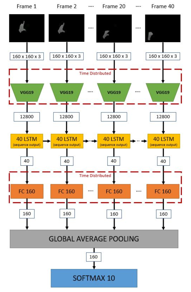
The Time Distribution operation applies the same operation for each frame in the input. The input to the model is a group of tensors (each video) of shape [frames, height, width, channels]. The chosen CNN transfer model receives a single frame at a time of shape [height, width, channels], which a 2D CNN can easily handle. The output of the CNN feeds into LSTM units. Depending on the number of units set in the config_default.yalm file, the LSTM layers try to learn many temporal relationships in consecutive frames. The output of CNN depends on the type of CNN model chosen during the training. For the Time Distributed VGG19 layer, the output tensor is of the dimension [frames, 12800] output from the 2D Maxpooling of each frame. This tensor is then fed into the LSTM layer, say with 40 units, which outputs a full sequence tensor (return_sequence = True)of shape [frames, 40]. This output tensor from the LSTM is then fed into a Time-Distributed Fully Connected layer with, say, 160 neurons. The output from the FC layer is [frames, 160]. This output tensor is then passed through the GlobalAveragePooling Layer, which outputs a tensor of size [160]. This tensor is then passed thru the SoftMax Layer with N classes, as illustrated in Figure 2. A significant amount of time was spent in getting this architecture to work. Although the Time Distribution Layer in Keras is helpful, the actual implementation requires a strong understanding of each functional component. Several different but similar architectures were tried before finalizing the one shown in Figure 2. For example, setting return_sequence = Falseoutputs a tensor of [40] rather than a tensor of [40, 40] which does not need a GlobalAveragePooling layer. The training loss and accuracy curves are saved to the ./report folder.
SETTING UP CONFIG FILES
A YAML-based configuration file was set up to manage hyperparameter tuning better using GridSearch. Python’s argparse library was used to load hyperparameters during training and testing execution. The YAML file can be found in the ./config folder. The YAML file can be easily edited to change various hyperparameters, including the choice of CNN transfer model, number of LSTM units, number of neurons in the FC layer, etc.
TESTING & PERFORMANCE MATRICES
The testing is implemented in Python Script test.py. The testing follows the same preprocessing step as that of the train. During training, the resulting model is saved in the /.model folder. While testing, this load model is loaded, and the output labels are predicted. The accuracy is printed to the console, and the Confusion Matrix, as a heatmap using the Seaborn library, is saved to the folder ./report.
EXPERIMENTS & RESULTS
The primary indicator of the model’s performance used on the project was Accuracy, followed by Confusion Matrix. Hyperparameters were tuned using the principles of Grid Search. The congif_default.yaml file has the baseline parameters used during Grid Search. In essence, one parameter was varied while others remained fixed. Table 1 shows all the hyperparameters that were part of the tuning scope.
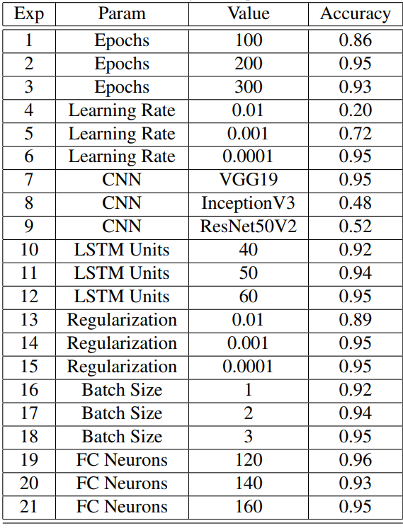
One of the most important decisions that needed to be made was the type of CNN architecture to use in the model. Three different architectures were experimented with: VGG19, InceptionV3, and ResNet50V2. Of all the architectures tested, VGG19 was found to produce the best results. This is not surprising as VGG19 is one of the most popular image recognition architectures. It surpasses baselines on many tasks and datasets beyond ImageNet. Although it does not have the lowest number of parameters compared with other architectures, its structure is fairly simple and uniform.
After the CNN architecture was established, experiments were conducted with different parameter values to understand their impact on the model’s performance. The tuned parameters were: No. of epochs, learning rate, RNN size, Regularization coefficient, batch_size, and frame size.
At 200 epochs, the best results were achieved. Although 300 epochs were tested, the accuracy dipped a bit below 200. The higher number of epochs in this case likely results in a model that has slightly over-fit on the training data, which causes a dip in the validation accuracy. This suggests that increasing the number of epochs beyond a “sweet spot” leads to diminishing returns.
Learning rate is one of the most important parameters in any Machine Learning model. In this application, the learning rate varied from 0.01 to 0.0001. The best results were produced from a learning rate of 0.0001. At such a small learning rate, the model updates the weights gradually over time until a stable set of weights is reached. The higher learning rates are trying to get the model to converge more quickly but are likely resulting in suboptimal weights, hence the lower accuracy.
The number of RNN units varied from 40 to 60. The higher the number of units, the better the model's performance. This result makes sense because more RNN units in the model correspond to more temporal features that get extracted. This especially helps the model differentiate between similar gestures that could confuse one another.
Regularization is a parameter commonly used in many machine learning models to reduce the likelihood of overfitting the training data. In this work, the regularization coefficient varied from 0.01 to 0.0001. It was observed that a little bit of regularization (0.0001) works best. When the regularization coefficient is too high, it has the effect of not generalizing the model sufficiently enough, which results in slightly lower accuracy.
The batch size determines the number of samples to use in each training cycle. The batch sizes tested were from 1 to 3. The batch size directly impacts the model’s training time; the larger the batch size, the longer the training time. Hence, in the interest of time, the batch sizes were kept fairly small. The accuracy from a batch size 2 and 3 was comparable, as shown in the results table. A batch size of 1 did not perform well because larger batch sizes have a regularization effect.
The last parameter tested was the hidden size of the fully connected layer. This parameter was varied from 120 to 160, of which the former produced the best results. The reason for this is that the larger, fully connected layer likely caused overfitting that caused a slight reduction in the accuracy of the test set.
The final set of parameters are fixed for the model are tabulated in Table 2.
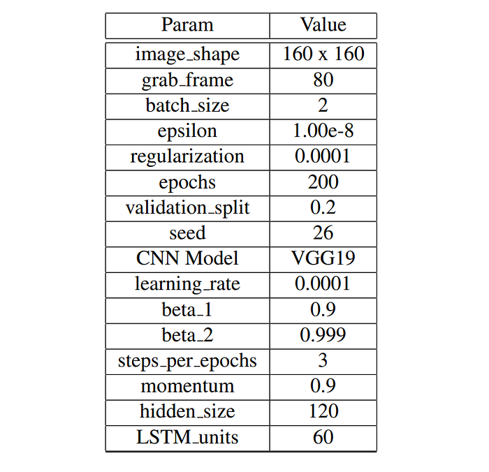
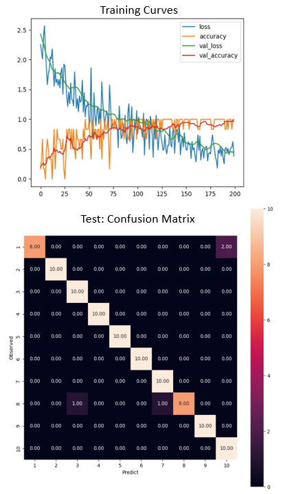
Figure 3 shows the training performance curves and the confusion matrix for the final model after hyperparameter tuning. The first thing we notice about the learning curve is that it’s choppy. This is expected as the batch size used during the training is very small. The smaller batch sizes helped with GPU resources in completing the training without running out of memory. In general, the learning loss and accuracy curves follow the general trends. Also, the confusion matrix shows higher confidence levels in classifying most of the classes accurately. However, there is some ambiguity in classifying Class 1, which the models predict as Class 10, 20 of the time. When we observe the gestures in Class 1 and Class 10 videos, we can see that they have very similar temporal features. This could be improved by providing more importance to spatial feature extraction in the CNN layer. One way to achieve this is by increasing the frame size to more than 160x160 so that there is enough area for convolution to extract better spatial features.
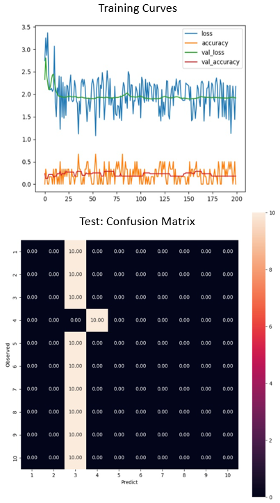
The learning rate plays a significant role in training a Time Distributed CNN-LSTM model. As seen in Figure 4, the loss curves quickly stagnate at local minima, and the accuracy does not improve. It is also seen in the confusion matrix that that model does not accurately predict the results. The influences of each hyperparameter presented in Table 1 are documented in an excel file and are available as supporting documents in the GitHub repository.
REFERENCES
[1] Kripesh Adhikari, Hamid Bouchachia, and Hammadi Nait-Charif. Activity recognition for indoor fall detection using a convolutional neural network. In 2017 Fifteenth IAPR Inter-National Conference on Machine Vision Applications (MVA),pages 81–84, 2017.
[2] hthuwal. Python video to frame, 2018. https://github.com/hthuwal/sign-language-gesture-recognition/blob/master/video-to-frame.py.
[3] User Kinght. How to detect two different colors using ‘cv2.inrange‘ in python-opencv?, 2018. https://stackoverflow.com/questions/48109650/how-to-detect-two-different-colors-using-cv2-inrange-in-python-opencv.
[4] Sarfaraz Masood, Adhyan Srivastava, Harish ChandraThuwal, and Musheer Ahmad. Real-time sign language gesture (word) recognition from video sequences using CNN and rnn. In Vikrant Bhateja, Carlos A. Coello Coello, Suresh Chandra Satapathy, and Prasant Kumar Pattnaik, edi-
tors, Intelligent Engineering Informatics, pages 623–632, Singapore, 2018. Springer Singapore.
[5] metal3d. A video frame generator respecting keras.sequence
class with data augmentation capacities, 2019. https:
//gist.github.com/metal3d/f671c921440deb93e6e040d30dd8719b.
[6] Michael0x2a. I need to write a python script to sort pictures, how would i do this?, 2013. https://stackoverflow.com/questions/23178039/i-need-to-
write-a-python-script-to-sort-pictures-how-would-i-do-this.
[7] Amit Moryossef. Developing real-time, automatic sign language detection for video conferencing, 2020. https://ai.googleblog.com/2020/10/developing-real-time-
automatic-sign.html.
[8] Franco Ronchetti, Facundo Quiroga, Cesar Estrebou, Laura Lanzarini, and Alejandro Rosete. Lsa64: A dataset of argentinian sign language. XX II Congreso Argentino de Ciencias de la Computaci ́on (CACIC), 2016.
[9] Arifa Sultana, Kaushik Deb, Pranab Kumar Dhar, and Takeshi Koshiba. Classification of indoor human fall events using deep learning. Entropy, 23(3):1–20, Mar. 2021. Publisher Copyright: © 2021 by the authors. Licensee MDPI, Basel, Switzerland.